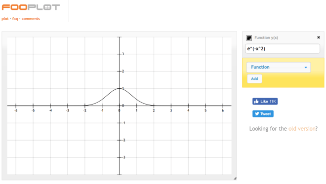
Lesson 49 – Symmetry: The language of normal distribution

Hello.

I am the normal distribution.

I am one of the most important density functions in probability. People are so used to me, almost to the point of using me for approximating any data.

You have seen in Lesson 47 and Lesson 48 that I am a good approximation for the distribution function of the sum of independent random variables. The Central Limit Theorem.

My functional form is

 f(x) = \frac{1}{\sqrt{2 \pi \sigma^{2}}} e^{\frac{-1}{2}(\frac{x-\mu}{\sigma})^{2}}

Did you notice I am merely a symmetric function e^{-x^{2}}, with some constants and parameters?

x can be positive or negative real numbers (continuous random variable)  -\infty < x < \infty .

\mu and \sigma are my control parameters.

Can you tell me what lesson was it where we learn that \mu is the mean or expected value and \sigma is the standard deviation of the distribution?

People use the notation N(\mu, \sigma) to say that I am a normal distribution with mean \mu and standard deviation \sigma.

\mu is my center. It can be positive or negative (-\infty < \mu < \infty), and the function is symmetric to its right and left. \sigma is how spread out I am from the center. It is positive (\sigma > 0).

Look at this example. I am centered on 60 and changing the spread. Narrow and wide flanks. Larger standard deviation results in a wider distribution with more spread around the mean.

In this example, I have the same spread, but I am changing my location (center).

I told you before that I am symmetric around the mean. So the following properties hold for me.

P(X > \mu) = P(X < \mu) = 0.5

P(X > \mu + a) = P(X < \mu - a)

f(\mu + a) = f(\mu-a)

By the way, if I give you the values for \mu and \sigma, do you know how to compute P(X \le x)?

You guessed it correct. Take my probability density function and integrate it from -\infty to x.

P(X \le x) = \int_{-\infty}^{x}\frac{1}{\sqrt{2 \pi \sigma^{2}}} e^{\frac{-1}{2}(\frac{x-\mu}{\sigma})^{2}}dx

For example,

Is this the cumulative distribution function  F(x)?

Compute the closed form solution of this integral.

P(X \le x) = \int_{-\infty}^{x}\frac{1}{\sqrt{2 \pi \sigma^{2}}} e^{\frac{-1}{2}(\frac{x-\mu}{\sigma})^{2}}dx

You can try change of variables method or the substitution method.

You can try integration by parts.

You can find the anti-derivative and use the fundamental theorem of calculus to solve.

I dare you to compute this integral to a closed form solution by next week.

We will continue our lessons after your tireless effort on this 😉

If you find this useful, please like, share and subscribe.
You can also follow me on Twitter @realDevineni for updates on new lessons.

Lesson 48 – Normal is the limit

What is this? Is it normal?

The shape is limited to a bell. Is it normal?

It is the same for any variable. Is it normal?

Why is it normal?

What is the normal?

The binomial distribution is the number of successes in n trials. It is the sum of n Bernoulli random variables.

S_{n} = X_{1} + X_{2} + ... + X_{n}, where  X_{i} \in (0,1) \hspace{5} \forall i

A mathematical approximation for the binomial distribution with a large number of trials is the Poisson distribution. We know that the average number of events in an interval ( \lambda ) is the expected number of successes np.

The wait time for the ‘r’th arrival follows a Gamma distribution. Gamma distribution is the sum of r exponential random variables.

 T_{r} = t_{1} + t_{2} + t_{3} + ... + t_{r}

What you observed in the animations last week, and what you saw now for the Binomial, Poisson, and Gamma as examples, is that the sum of random variables is tending towards a particular shape (distribution function).

This observation is “central” to probability theory.

It is called the Central Limit Theorem.

If S_{n} is the sum of  n independent random variables, then the distribution function of  S_{n} can be well-approximated by a continuous function knows as the normal density function given by

f(x) = \frac{1}{\sqrt{2 \pi \sigma^{2}}} e^{\frac{-1}{2}(\frac{x-\mu}{\sigma})^{2}}

where  \mu and \sigma^{2} are the expected value and variance of the original distribution.

It was first proved by a French mathematician Abraham de Moivre in the early 1700s. He showed this in one of the chapters of his thesis, The Doctrine of Chances. Page 243: “A Method of approximating the Sum of the Terms of the Binomial  (a+b)^{n} expanded into a Series, from whence are deduced some practical Rules to estimate the Degree of Assent which is to be given to Experiments.

An interesting observation from his thesis.

As you can see, he derived useful approximations to Binomial series. Imagine computing factorials for large values of n in those times.

It turns out that the binomial distribution can be estimated very accurately using the normal density function.

 f(x) = \frac{n!}{(n-x)!x!}p^{x}(1-p)^{n-x} = \frac{1}{\sqrt{2 \pi \sigma^{2}}} e^{\frac{-1}{2}(\frac{x-\mu}{\sigma})^{2}}

I compiled the modern version of this derivation. It is long with all the steps.

Please CLICK HERE to read and understand the details.

Follow it through the end. You will feel good to see how Binomial converges in the limit to this symmetric distribution.

Most probability distributions are related some way or the other to independent Bernoulli trails (the root events). If you carefully look at the probability distribution functions for each of them and take it to the limit as n \rightarrow \infty, you will see how the normal distribution emerges as the limiting distribution.

That is why it is normal.

The intuition from convolution

A very intuitive and elegant way of understanding the Central Limit Theorem and why the bell shape emerges due to convergence in the center of the distribution is provided in Chapter 9 (Preasymptotic and Central Limit in the Real World) of Silent Risk, technical notes on probability by Nassim Nicholas Taleb.

The gist is as follows.

We are deriving the distribution function for the summation of the random variables.

S_{n} = X_{1} + X_{2} + ... + X_{n}

You know from lesson 46 that this is convolution.

If X and Y are two independent random variables with probability density functions f_{X}(x) and f_{Y}(y), their sum Z = X + Y is a random variable with a probability density function f_{Z}(z) that is the convolution of f_{X}(x) and f_{Y}(y).

 f(z) = f_{X}*f_{Y}(z) = \int_{-\infty}^{\infty}f_{X}(x)f_{Y}(z-x)dx

Convolution is the multiplication of functions.

The probability distribution (for example, f_{Y}(z-x)) is weighted using another function (for example, f_{X}(x)). When we repeat this through induction, we smooth out the function at the center till it gets a bell-like shape and the tails become thin.

In Chapter 9, he provides an example convolution of uniform random variables.

Convolution of two uniform random variables (S_{n} = X_{1} + X_{2} ) is a triangular function (piecewise linear).

Convolution of this triangular function with another uniform random variable (rectangular function) (S_{n} = S_{n-1} + X_{3} ) will now yield a quadratic function.

As the samples grow (n becomes large), these function multiplications yield a smooth center heavy and thin tailed bell function — the normal density.

Look at this animation. See how the uniform rectangular function X_{1} becomes a triangle (X_{1} + X_{2}) and quickly converges to a normal density for n = 5.

This one is for the sum of Poisson random variables.

Notice that even for n = 10, the distribution is not fully normal. It is not converging fast. And that is important to remember.

While the Central Limit Theorem is central to the probability theory, and it is a fundamental assumption for many concepts we will learn later, we should know that some distributions converge quickly, some do not.

We will learn about the normal distribution in detail in the next few lessons. As you prepare for the normal distribution, I will leave you with a comment posted last week about the normal distribution by a good friend who works in the insurance industry.

“As has been shown time and again, there is no such thing as a ‘normal’ distribution in the real world -;)”

Well, what can I say, he works on real work risk with real dollars at stake. Always take the word of a person who has skin in the game.

If you find this useful, please like, share and subscribe.
You can also follow me on Twitter @realDevineni for updates on new lessons.

Lesson 47 – Is it normal?

The wait time for the first/next arrival follows an Exponential distribution. The wait time for the ‘r’th arrival ( T_{r} = t_{1} + t_{2} + t_{3} + ... + t_{r} ) follows a Gamma distribution.

The probability density function of the Gamma distribution is derived using the convolution of individual random variables  t_{1}, t_{2}, ... t_{r} .

 f(t) = \frac{\lambda e^{-\lambda t}(\lambda t)^{r-1}}{(r-1)!}

For increasing values of r, the distribution is like this.

It tends to look like a bell. Is it normal?

Nah, it may be a Gamma thing. Let me add uniform distributions.

 f(x) = 1 \forall 0 < x < 1

For increasing values of n, the distribution of the sum of the uniform random variables is like this.

It tends to look like a bell. Is it normal?

Hmm. I think it is just a coincidence. I will check Poisson distribution for increasing values of \lambda. Afterall, it is a discrete distribution.

P(X=x) = \frac{e^{-\lambda t}(\lambda t)^{x}}{x!}; x = 0, 1, 2, ...

Tends to look like a bell. Is it normal?

Perhaps coincidence should concede to a consistent pattern. If this is a pattern, does it also show up in the Binomial distribution?

P(X=x) = {n \choose x}p^{x}(1-p)^{n-x}; x = 0, 1, 2, ... n

There it is again. It looks like a bell.

What is this? Is it normal?

The shape is limited to a bell. Is it normal?

It is the same for any variable. Is it normal?

Why is it normal?

What is the normal?

To be continued…

If you find this useful, please like, share and subscribe.
You can also follow me on Twitter @realDevineni for updates on new lessons.

Lesson 46 – How convoluted can it be?

After last week’s conversation with Devine about Gamma distribution, an inspired Joe wanted to derive the probability density function of the Gamma distribution from the exponential distribution using the idea of convolution.

But first, he has to understand convolution. So he called upon Devine for his usual dialog.

J: Hello D, I can wait no longer, nor can I move on to a different topic when this idea of convolution is not clear to me. I feel anxious to know at least the basics that relate to our lesson last week.

D: It is a good anxiety to have. Will keep you focused on the mission. Where do we start?

J: We are having a form of dialog since the time we met. Why don’t you provide the underlying reasoning, and I will knit the weave from there.

D: Sounds good to me. Let me start by reminding you of our conversation in Lesson 23 about probability distribution. You introduced me to the Chicago dice game where you throw a pair of dice to score the numbers 2 – 12 in the order of the rounds.

J: Yes, I remember.

D: Let’s assume that Z is that outcome which is the sum of the numbers on each dice, say X and Y.

 Z = X + Y

Create a table of these outcomes and what combinations can give you those outcomes.

J: We did this too during lesson 23. Here is the table.

D: Now, take any one outcome for Z, let’s say Z = 3, and find out the probability that the random variable Z takes a value of 3, i.e., how do you compute P(Z = 3)?

J: There are two ways of getting a number 3, when X = 1 and Y = 2, or when X = 2 and Y = 1. The total combinations are 36, so P(Z = 3) = 2/36.

D: Excellent. Now let me walk you through another way of thinking. You said the there are two ways of getting a number 3.

X = 1 and Y = 2
or
X = 2 and Y = 1

What is the probability of the first combination?

J: P(X = 1 and Y = 2) = P(X = 1).P(Y = 2) since X and Y are independent.

D: What is the probability of the second combination?

J: P(X = 2 and Y = 1) = P(X = 2).P(Y = 1), again since X and Y are independent.

D: What is the probability of Z = 3 based on these combinations?

J: Ah, I see. Since either of these combinations can occur to get an outcome 3, P(Z = 3) is the union of these combinations.

P(Z = 3) = P(X = 1).P(= 2) + P(X = 2).P(Y = 1) = 2/36

D: Yes. If you represent these as their probability mass functions, you get

 f(z) = \sum_{all-possible-combinations} f(x)f(y)

Let me generalize it to any function of X and Y so that it can help in your derivations later.

We are attempting to determine f(z), the distribution function of Z. P(Z = z). If X = x, then for the summation Z = X + Y to be true, Y = zx.

This corollary means we can find out f(z) over all possible values of x as,

 P(Z = z) = \sum_{-\infty}^{\infty} P(X = x)P(Y=z-x)

 f(z) = \sum_{-\infty}^{\infty} f_{X}(x)f_{Y}(z-x)

This property is called the convolution of  f_{X}(x) and  f_{Y}(y).

J: Then, I suppose for the continuous distribution case it will be analogous. The summation will become an integration.

D: Yes. If X and Y are two independent random variables with probability density functions  f_{X}(x) and  f_{Y}(y), their sum Z = X + Y is a random variable with a probability density function f_{Z}(z) that is the convoluton of  f_{X}(x) and  f_{Y}(y).

 f(z) = f_{X}*f_{Y}(z) = \int_{-\infty}^{\infty}f_{X}(x)f_{Y}(z-x)dx

The density of the sum of two independent random variables is the convolution of their densities.

The exact mathematical proof can also be derived, but maybe we leave that to a later conversation.

J: Understood. But like all basics, we saw this for two random variables. How then, can we extend this to the sum of n random variables. I am beginning to make connections to the Gamma distribution case that has the sum of n exponential random variables.

D: That is a good point. Now let’s suppose  S_{n} = X_{1} + X_{2} + ... + X_{n} is the sum of n independent random variables. We can always rewrite this as S_{n} = S_{n-1} + X_{n} and find the probabilty distribution function of S_{n} through induction.

J: Got it. It seems to follow the logic. Now, let me use this reasoning and walk through the derivation of the Gamma distribution.

D: Go for it. The floor is yours.

J: I will start with the two variable case. Our second meeting happened at lesson 9, and the time to the second arrival from the origin is  T_{2} = t_{1} + t_{2} = 9.

The random variable  T_{2} is the sum of two random variables  t_{1} and  t_{2} . I want to determine the probability density function of  T_{2} . I will apply the convolution theory. For consistency with today’s notations, let me take  T_{2} = Z ,  t_{1} = X , and  t_{2} = Y .

f_{Z}(z) = f_{X}*f_{Y}(z) = \int_{-\infty}^{\infty}f_{X}(x)f_{Y}(z-x)dx

f_{Z}(z) = f_{X}*f_{Y}(z) = \int_{0}^{z}\lambda e^{-\lambda x}\lambda e^{-\lambda (z-x)} dx

Both X and Y are bounded at 0, and if this is true,  y \ge 0 implies  x \le z, and  x \ge 0 implies  y \le z. Either way, the limits of the integral are from 0 to z.

f_{Z}(z) = f_{X}*f_{Y}(z) = \int_{0}^{z}\lambda^{2} e^{-\lambda x} \frac{e^{-\lambda z}}{e^{-\lambda x}} dx

f_{Z}(z) = f_{X}*f_{Y}(z) = \lambda^{2} e^{-\lambda z} \int_{0}^{z} dx

f_{Z}(z) = f_{X}*f_{Y}(z) = \lambda^{2} z e^{-\lambda z}

D: Excellent. Let me show how this function looks.

Do you see how the Gamma distribution is evolving out of exponential distribution?

J: Yes. Very clear.

D: Continue with your derivation.

J: For a three variable case, I will assume P = X + Y + S. I can also write this as P = Z + S analogous to  S_{n} = S_{n-1}+X_{n} .

Then I have the distribution function of P as

f_{P}(p) = f_{Z}*f_{S}(p) = \int_{0}^{p}\lambda^{2} z e^{-\lambda z} \lambda e^{-\lambda (p-z)} dz

f_{P}(p) = f_{Z}*f_{S}(p) = \lambda^{3} \int_{0}^{p}z e^{-\lambda z}\frac{e^{-\lambda p}}{e^{\lambda z}} dz

f_{P}(p) = f_{Z}*f_{S}(p) = \lambda^{3} e^{-\lambda p} \int_{0}^{p} z dz

f_{P}(p) = f_{Z}*f_{S}(p) = \lambda^{3} e^{-\lambda p} \frac{p^{2}}{2}

We can rewrite this as

f_{P}(p) = f_{Z}*f_{S}(p) = \frac{\lambda e^{-\lambda p} (\lambda p)^{(3-1)}}{(3-1)!}

so that the general Gamma distribution function for n variables becomes,

 f(t) = \frac{\lambda e^{-\lambda t}(\lambda t)^{r-1}}{(r-1)!}

D: Joe that is some well thought out derivation. You are really into this data analysis stuff now.

J: 😎 😎 Do we have anything else to cover today?

D: Using the same logic, can you derive the distribution for the sum of normals?

J: Normals? 😕 😕 😕


Oops, I think that is for the next week.
Don’t you have to get ready for the new year parties? It may be the coldest New Year’s eve on record. So you better bundle up!

Happy New Year.

If you find this useful, please like, share and subscribe.
You can also follow me on Twitter @realDevineni for updates on new lessons.

Lesson 45 – Time to ‘r’th arrival: The language of Gamma distribution

Joe and Devine Meet Again — for the ‘r’th time

J: It’s been 13 lessons since we met last time. Thought I’d say hello. You did not show up last week. I kept waiting as you asked me to in lesson 44.

D: Hey Joe! Sorry for the wait. I had a tough choice between travel/work and the weekly lesson. Could only do one. It was not intentional, although where we left off kind of hinted toward the wait. End of the year is a busy time for all.

J: I noticed you covered exponential distribution and its memoryless property in the previous two lessons. Isn’t time to our meetings also exponential?

D: That is correct. The first time we met was in lesson 6. The wait time  t_{1} was 6. We met again in lesson 9. The wait time (or wait lessons)  t_{2} was 3. Between the last time we met and now, as you pointed out, the wait time  t_{8} is 13. In lesson 43, where we first discussed the exponential distribution, I showed how its probability density function is derived. Did you follow the logic there?

J: Yes, I did. We begin with the fact that the arrival time (to the first or next event) exceeds some value t only if there are no events in the interval [0, t].

The probability that T > t is equal to the probability that there are 0 events in the period. P(N = 0) is computed from the Poisson distribution.

 P(T > t) = P(N = 0) = \frac{e^{-\lambda t}(\lambda t)^{0}}{0!} = e^{-\lambda t}

Since  P(T > t) = e^{-\lambda t} ,  P(T \le t) = 1 - e^{-\lambda t}.

 P(T \le t) is the cumulative density function  F(t) for the exponential distribution.

We can get the probability density function f(t) by taking the derivative of F(t).

 f(t) = \frac{d}{dt}F(t) = \frac{d}{dt}(1-e^{-\lambda t}) = \lambda e^{-\lambda t}

D: Well done. The inter-arrival time follows an exponential probability distribution.

J: Isn’t the exponential distribution like the Geometric distribution? I learned in lesson 33 that the random variable which measures the number of trials it takes to see the first success is Geometrically distributed.

D: That is a shrewd observation. Yes, the exponential distribution is the continuous analog of the discrete geometric distribution.

In geometric distribution, the shape is controlled by p, the parameter. The greater the value of p, the steeper the fall.

In exponential distribution, the shape is controlled by  \lambda .

J: In that case, does the exponential distribution also have a related distribution that measures the wait time till the ‘r’th arrival?

D: Can you be more specific?

J: The geometric distribution has the Negative binomial distribution that measures the number of trials it takes to see the ‘r’th success. Remember lesson 35?

Just like the exponential distribution is the continuous analog of the discrete geometric distribution, is there a continuous analog for the discrete negative binomial distribution?

D: Yes, there is a related distribution that can be used to estimate the time to the ‘r’th arrival. It is called the Gamma distribution.

Look at our timeline chart for instance. The time to the first arrival is t_{1} = 6 . The time to the second arrival since the first arrival is t_{2} = 3 . But, our second meeting happened at lesson 9, so the time to the second arrival from the origin is  T_{2} = t_{1} + t_{2} = 9 .

Similarly, the second time we meet again after lesson 9 is in lesson 16. So, the time to the second arrival since lesson 9 is 16 – 9 = 7. Put together, these times to second meeting follow a Gamma distribution. More generally,

the wait time for the ‘r’th arrival follows a Gamma distribution.

J: That seems to be a logical extension. I believe we can derive the probability density function for the Gamma distribution using the exponential distribution. They seem to be related. Can you help me with that?

D: Sure. If you noticed, I said that our second meeting happened at lesson 9, and the time to the second arrival from the origin is  T_{2} = t_{1} + t_{2} = 9 .

J: Yes. That is because it is the total time — the first arrival and the second arrival since.

D: So the random variable  T_{2} is the sum of two random variables  t_{1} and  t_{2}

The time to ‘r’th arrival  T_{r} = t_{1} + t_{2} + t_{3} + ... + t_{r}.

We can derive the probability density function of  T_{r} using the convolution of the individual random variables t_{1}, t_{2}, ... t_{r} .

J: 😕 What is convolution?

D: It might require a full lesson to explain it from first and show some examples, but for now remember that convolution is the blending of two or more functions. If you have two continuous random variables X and Y with probability density functions f(x) and  g(y) , then, the probability density function of the new random variable Z = X + Y is

 (f*g)(z) = \int_{-\infty}^{\infty}f(z-y)g(y)dy

Employing this definition on r variables ( t_{1}, t_{2}, ..., t_{r}) using induction, we can get the probability density function of the Gamma distribution as

 f(t) = \frac{\lambda e^{-\lambda t}(\lambda t)^{r-1}}{(r-1)!}

J: 😕 😕 😕   😕 😕 😕

D: Not to worry. We will learn some of the essential steps of convolution soon.

J: I have to say, the density function looks a little convoluted though. 😉

D: Ah, that’s a good one. Perhaps it is. Why don’t you check what happens to the equation when you choose r = 1, i.e., the arrival time for the first event.

J: Let me try.  f(t) = \lambda e^{-\lambda t} . This is the density function for the exponential distribution. It has to, because we measure the arrival time to the first event.

D: You are correct. The Gamma distribution has two control parameters. \lambda is called the scale parameter because it controls the width of the distribution and r is called the shape parameter because it controls the shape parameter.

J: Can we make some quick graphics to see how the distribution looks.

D: Yes, here it is. This one is for a  \lambda of 0.2 and r changes from 1 to 4, i.e., for use to meet the first time, second time, third time and the fourth time.

J: This is cool. I see that the tails are getting bigger as the value of r increases.

D: Good observation again. That is why Gamma distribution is also used to fit data with significant skewness. It is widely used for fitting rainfall data. Insurance agents also use it to model the claims.

J: Understood. When do we meet again? We have to figure out the convolution stuff.


You now have all the tools to estimate this. Figure out the probability that the wait time is more than one week while we celebrate the emergence of the light from darkness.

Merry Christmas.

If you find this useful, please like, share and subscribe.
You can also follow me on Twitter @realDevineni for updates on new lessons.

Lesson 44 – Keep waiting: The memoryless property of exponential distribution

Bob Waits for the Bus

As the building entrance door closes behind, Bob glances at his post-it note. It has the directions and address of the car dealer. Bob is finally ready to buy his first (used) car. He walks to the nearby bus stop jubilantly thinking he will seldom use the bus again. Bob is tired of the waiting. Throughout these years the one thing he could establish is that the average wait time for his inbound 105 at the Cross St @ Main St is 15 minutes.

Bob may not care, but we know that his wait time follows an exponential distribution that has a probability density function  f(t) = \lambda e^{-\lambda t} .

The random variable T, the wait time between buses is an exponential distribution with parameter  \lambda . He waits 15 minutes on average. Some days he boards the bus earlier than 15 minutes, and some days he waits much longer.

Looking at the function  f(t) = \lambda e^{-\lambda t} , and the typical information we have for exponential distribution, i.e., the average wait time, it will be useful to relate the parameter  \lambda to the average wait time.

The average wait time is the average of the distribution — the expected value E[.].

E[X] for a continuous distribution, as you know from lesson 24 is  E[X] = \int x f(x) dx.

Applying this using the limits of the exponential distribution, we can derive the following.

 E[T] = \int_{0}^{\infty} t f(t) dt

 E[T] = \int_{0}^{\infty} t \lambda e^{-\lambda t} dt

 E[T] = \lambda \int_{0}^{\infty} t e^{-\lambda t} dt

The definite integral is  \frac{1}{\lambda^{2}} .

So we have

E[T] = \frac{1}{\lambda}

The parameter  \lambda is a non-negative real number ( \lambda > 0), and represents the reciprocal of the expected value of T.

In Bob’s case, since the average wait time (E[T]) is 15 minutes, the parameter \lambda is 0.066.

Bob gets to the bus shelter, greets the person next to him and thinks to himself “Hope the wait will not exceed 10 minutes today.”

Please tell him the probability he waits more than 10 minutes is 0.5134.

 P(T > 10) = e^{-\lambda t} = e^{-10/15} = 0.5134

Bob is visibly anxious. He turns his hand and looks at his wristwatch. “10 minutes. The wait won’t be much longer.”

Please tell him about the memoryless property of the exponential distribution. The probability that he waits for another ten minutes, given he already waited 10 minutes is also 0.5134.

Let’s see how. We will assume t represents the first ten minutes and s represents the second ten minutes.

 P(T > t + s \mid T > t) = \frac{P(T > t \cap T > t+s)}{P(T > t)}

\hspace{10cm} = \frac{P(T > t+s)}{P(T > t)}

\hspace{10cm} = \frac{e^{-\lambda (t+s)}}{e^{-\lambda t}}

\hspace{10cm} = \frac{e^{-\lambda t} e^{-\lambda s}}{e^{-\lambda t}}

\hspace{10cm} = e^{-\lambda s}

 P(T > 10 + 10 \mid T > 10) = e^{-10\lambda} = 0.5134

The probability distribution of the remaining time until the event occurs is always the same regardless of the time that passed.

There is no memory in the process. The history is not relevant. The time to next arrival is not influenced by when the last event or arrival occurred.

This property is unique to the strictly decreasing functions: exponential and the geometric distributions.

The probability that Bob has to wait another s minutes (t + s) given that he already waited t minutes is the same as the probability that Bob waited the first s minutes. It is independent of the current wait time.

Bob Gets His First Chevy

Bob arrives at the dealers. He loves the look of the red 1997 Chevy. He looks over the window pane; “Ah, manual shift!” That made up his mind. He knows what he is getting. The price was reasonable. A good running engine is all he needed to drive it away.

The manager was young, a Harvard alum, as Bob identified from things in the room. “There is no guarantee these days with academic inflation, … the young lad is running a family business, … or his passion is to sell cars,” he thought to himself.

The manager tells him that the engine is in perfect running condition and the average breakdown time is four years. Bob does some estimates ($$$$) in his mind while checking out the car. He is happy with what he is getting and closes the deal.

Please tell Bob that there is a 22% likelihood that his Chevy manual shift will break down in the first year.

The number of years this car will run ~ exponential
distribution with a rate (\lambda) of 1/4.

Since the average breakdown time (expected value E[T]) is four years, the parameter \lambda = 1/4.

 P(T \le 1) = 1 - e^{-\lambda t} = 1 - e^{-(1/4)} = 0.22

Bob should also know that there is a 37% chance that his car will still be running fine after four years.

P(T > 4) = e^{-4\lambda} = e^{-4/4} = 0.37

Bob in Four Years

Bob used the car for four years now with regular servicing, standard oil changes, and tire rotations. The engine is great.

Since the average lifetime has passed, should he think about a new car? How long should we expect his car to continue without a breakdown? Another four years?

Since he used it for four years, what is the probability that there will be no breakdown until the next four years?

You guessed it, 37%.

 P(T > 8 \mid T > 4) = \frac{P(T > 8)}{P(T > 4)} = e^{-4\lambda} = 0.37

Now let’s have a visual interpretation of this memoryless property.

The probability distribution of the wait time (engine breakdown) for  \lambda = 1/4 looks like this.

Let us assume another random variable  T_{2} = T - 4, as the breakdown time after four years of usage. The lower bound for  T_{2} is 0 (since we measure from four years), and the upper bound is \infty.

For any values  T > 4 , the distribution is another exponential function — it is shifted by four years.

 f(t_{2}) = \lambda e^{-\lambda t_{2}} = \lambda e^{-\lambda (t-4)}

Watch this animation, you will understand it better.

The original distribution is represented using the black line. The conditional distribution  P(T > 4+s \mid T > 4) is shown as a red line using links.

The same red line with links (truncated at 4) is shown as the shifted exponential distribution (f(t_{2})=\lambda e^{-\lambda (t-4)}). So, the red line with links from t = 4 is the same as the original function from t = 0. It is just shifted.

The average value of T is four years. The average value of T_{2} = T - 4 is also four. They have the same distribution.

If Bob reads our lessons, he’d understand that his Chevy will serve him, on the average, another four years.

Just like the car dealer’s four-year liberal arts degree from Harvard is forgotten, Bob’s four-year car usage history is forgotten — Memoryless.

As the saying goes, some memories are best forgotten, but the lessons from our classroom are never forgotten.

If you find this useful, please like, share and subscribe.
You can also follow me on Twitter @realDevineni for updates on new lessons.

Lesson 43 – Wait time: The language of exponential distribution

Wednesday, no, the Waiting Day

November 29, 2017

6:00 AM

As the cool river breeze kisses my face, I hear the pleasant sound of the waves. “How delightful,” I think, as I drop into the abyss of eternal happiness. The sound of the waves continues to haunt me. I run away from the river; the waves run with me. I close my ears; the waves are still here.

It’s the time when your dream dims into reality. Ah, it’s the sound of the “waves” on my iPhone. Deeply disappointed, I hit the snooze and wait for my dream to come back.

6:54 AM

“Not again,” I screamed. I have 30 minutes to get ready and going. I-95 is already bustling. I can’t afford to wait long in the toll lane. Doctor’s check-in at 8 AM.

7:55 AM

“Come on, let’s go.” For the 48th time, waiting in the toll lane, I curse myself for not having gotten the EZ pass that week. “Let’s go, let’s go.” I maneuver my way while being rude to the nasty guy who tried to sneak in front of my car. Finally, I pay cash at the toll and drive off in a swift to my doctor’s.

8:15 AM

“Hi, I have an appointment this morning. Hope I am not late.” The pretty lady at the desk stared at me, gave me a folder and asked me to wait. Dr. D will be with you shortly. As I was waiting for my turn, I realized that the lady’s stare was for my stupid question. My appointment was at 8 AM after all.

8:50 AM

The doctor steps in; “Please come in” he said. A visibly displeased me walked-in instantly, all the way shaking my head for the delay. My boss will be waiting for me at the office. We are launching a new product today.

9:15 AM

“You are in perfect health. The HDLs and LDLs are normal. Continue the healthy eating and exercise practices you have. See you next time, but don’t wait too long for the next visit.”

9:25 AM

My wait continues, this time for the train. “The next downtown 1-train will arrive in 10 minutes,” said the man (pre-recorded).

10:00 AM

My boss expressed his displeasure at my delay in his usual sarcastic ways. “But, I told you I was going to be late today,” I said to myself. We get busy with work and the product launch.

1:00 PM

I am waiting in the teller line at the local bank. Essential bank formalities and some checks to deposit. There were already ten people before me; there is only one teller, and for some reason, she is taking her own sweet time to serve each customer.

The only other living being in the bank (bank employees of course) is the manager; she is busy helping a person with his mortgage. “Poor guy seems to be buying a house at the peak,” I thought as I start counting the time it is talking to serve each customer.

1:35 PM

“One extra-hot Cappuccino,” said Joe at Starbucks in his usual stern voice. The wait for my coffee was not as annoying. There’s something about coffee and me. Can wait forever ! or maybe it is Starbucks; I can’t say.

7:00 PM

After a long tiring, waiting day, I am still waiting for my train.

I waited 22 minutes. The train surely has to come in the next minute,” I said to myself.

The clock ticks, my energy drops, still no trail.

.

.

.

“The next uptown 1-train is now arriving. Please stand away from the platform edge.”

I step in and grab the one remaining seat. “Finally; no more waiting for the day,” I said to myself.

The wheels rattle, the brains muffle, and the eyes scuttle. Same beautiful abyss of happy, restful state from the morning.

8:00 PM

As I park my car and check my door mail, I realize that my day was filled with wait times. I said to myself, “Aren’t these the examples of exponential distribution that data analysis guy from college used to talk about? I finally understand it. You live and learn.”

9:00 PM

I start logging my Wednesday, no, the waiting day.

“Let me derive the necessary functions for the exponential distribution before I go to bed,” I said to myself.

The time between arrivals at service facilitates, time to failure of systems, flood occurrence, etc., can be modeled as exponential distributions.

Since I want to measure the time between events, I should think of time T as a continuous random variable,  t_{1}, t_{2}, t_{3} , etc., like this.

That means, this distribution is positive only, as  T \ge 0 (non-negative real numbers).

We can have a small wait time or a long wait time. It varies, and we are estimating the probability that T is less than or greater than a particular time, and between two times.

The distribution of the probability of these wait times is called the exponential distribution.

As I watch the events and wait times figure carefully, I can sense that there is a relation between the Poisson distribution and the Exponential distribution.

The Poisson distribution represents the number of events in an interval of time, and the exponential distribution represents the time between these events.

If N is the number of events during an interval ( a span of time) with an average rate of occurrence \lambda,

P(N = k) = \frac{e^{-\lambda t}(\lambda t)^{k}}{k!}

If T is measured as the time to next occurrence or arrival, then it should follow an exponential distribution.

The time to arrival exceeds some value t, only if N = 0 within t, i.e., if there are no events in an interval [0, t].

 P(T > t) = P(N = 0) = \frac{e^{-\lambda t}(\lambda t)^{0}}{0!} = e^{-\lambda t}

If  P(T > t) = e^{-\lambda t} , then  P(T \le t) = 1 - e^{-\lambda t} .

I know that P(T \le t) = F(t) is the cumulative density function. It is the integral of the probability density function. F(t) = \int_{0}^{t}f(t)dt.

The probability density function f(t) can then be obtained by taking the derivative of F(t).

f(t) = \frac{d}{dt}F(t) = \frac{d}{dt}(1-e^{-\lambda t}) = \lambda e^{-\lambda t}

The random variable T, the wait time between successive events is an exponential distribution with parameter \lambda.

Let me map this on to the experiences I had today.

If on average, 25 vehicles pass the toll per hour, \lambda=25 per hour. Then the wait time distribution for the next vehicle at the toll should look like this.

The probability that I will wait more than 5 minutes to pass the toll is  P(T > 5) = e^{-\lambda t} = e^{-25*(5/60)} = 0.125.

So, the probability that my wait time will be less than 5 minutes is 0.875. Not bad. I should have known this before I swore at the guy who got in my way.

It is clear that the distribution will be flatter if \lambda is smaller and steeper if \lambda is larger.

10:00 PM

I lay in my bed with a feeling of accomplishment. My waiting day was eventful; I checked off all boxes on my to-do list. I now have a clear understanding of exponential distribution.

10:05 PM

I am hoping that I get the same beautiful dream. My mind is still on exponential distribution with one question.

“I waited 22 minutes for the train in the evening, why did it not arrive in the next few minutes? Since I waited a long time, shouldn’t the train arrive immediately?”

A tired body always beats the mind.

It was time for the last thought to dissolve into the darkness. The SHIREBOURN river is “waiting” for me on the other side of the darkness.

If you find this useful, please like, share and subscribe.
You can also follow me on Twitter @realDevineni for updates on new lessons.

Lesson 42 – Bounded: The language of Beta distribution

Last week, in Lesson 41, we started toying with the idea of continuous probability distributions. When a random variable X is continuous (i.e., can be any Real number), we can compute the probability of X between any two values,  P(X \in (a,b)) = P(a \le X < b) using a continuous probability distribution function  f(x) .

The continuous probability density function (pdf) is the limiting shape of the frequency plot (histogram) of the data as the number of possible observations (n) goes to infinity. While the probability that the random variable X takes any specific value x is 0, the height of the smooth curve measures how dense the probability is at that point.

In the limit, as the number of observations approaches infinity (continuous), the proportion of observations that belong to an interval (a, b) is the probability that X is in this interval;  P(X \in (a,b)) = P(a \le X < b) .

This area under the curve is computed using the integral of the function over the range a to b.

 P(a < X < b) = \int_{a}^{b} f(x) dx

I left you with a few practice questions:

If X is a random variable with a probability distribution function defined as

 f(x) = 90x^{8}(1-x) for 0 < x < 1

  1. What is the probability that X is between 0.2 and 0.3?
  2. What is the probability that X will exceed 0.9?
  3. What is the median of X?

If you have solved these questions, more power to you. If you are waiting for the stars to align, this is that auspicious moment!

Let’s solve this problem step by step to understand the nuts and bolts of continuous distributions. At the end of the problem, I will lead you to our first type of continuous probability distribution functions, the Beta distribution and its special case, the uniform distribution. You will see why I selected this problem as the primer.

Our function is  f(x) = 90x^{8}(1-x) for 0 < x < 1.

The plot of this function reveals a bell-like shape. Notice that x is between 0 and 1 and the function is continuous.

Let’s take the first question: What is the probability that X is between 0.2 and 0.3?

 P(0.2 < X < 0.3) = \int_{0.2}^{0.3} f(x) dx

 = \int_{0.2}^{0.3} 90x^{8}(1-x) dx

 = \int_{0.2}^{0.3}90x^8 dx - \int_{0.2}^{0.3}90x^{9}dx

 = \frac{90}{9} x^{9}\Big|_{0.2}^{0.3} - \frac{90}{10} x^{10}\Big|_{0.2}^{0.3}

 = \frac{90}{9}(0.3^{9}-0.2^{9}) - \frac{90}{10}(0.3^{10}-0.2^{10})

 = 0.00014

Using the same procedure, we can solve for the probability that X will exceed 0.9?

 P(X > 0.9) = \int_{0.9}^{1} f(x) dx

 = \frac{90}{9} x^{9}\Big|_{0.9}^{1} - \frac{90}{10} x^{10}\Big|_{0.9}^{1}

 = \frac{90}{9}(1^{9}-0.9^{9}) - \frac{90}{10} (1^{10}-0.9^{10})

 = 0.264

We could have integrated the function from 0 to 0.9 and then subtracted this number from 1 because  P(X > x) = 1 - P(X \le x) and  P(X \le x) = \int_{0}^{x}f(x)dx in this case.

Also, remember that  P(X \le x) = F(x), the cumulative distribution function. We will be using the cumulative distribution function very often from now on.

Now, let us look at the third question: what is the median of X?

We know from order statistics that median is the 50th percentile, i.e., the value for which 50% of the values of X are below this number.

 P(X \le x_{median}) = F(x_{median}) = 0.5

\int_{0}^{x_{median}}f(x)dx = 0.5

 \int_{0}^{x_{median}}90x^{8}(1-x)dx = 0.5

This reduces to  10x_{median}^{9} - 9x_{median}^{10} = 0.5

We can use the Newton Raphson iterative method to find that the root of this equation is 0.84 when 0 < x < 1.

Hence,  x_{median} = 0.84

Beta Distribution

Now, look at the function I gave you carefully.
 f(x) = 90x^{8}(1-x) for 0 < x < 1

It is bounded between 0 and 1.

It has some exponents for x and (1-x); 8 and 1 in this case.

It has a constant, 90, acting as a multiplier.

The function we solved is a Beta distribution. The standard form, i.e., the probability density function of a Beta distribution is

 f(x) = cx^{a-1}(1-x)^{b-1} for 0 < x < 1.

As you can see, it is defined only in the 0 to 1 range. The beta distribution is a bounded distribution. The function is 0 everywhere else.

a and b are the parameters that control the shape of the distribution. They can take any positive real numbers; a > 0 and b > 0. In our example, a = 9 and b = 2. The distorted bell shape we have for the function is because of these two values.

c is called the normalizing constant. It ensures that the pdf integrates to 1. Take, for example, our function  f(x) = 90x^{8}(1-x) .

If we integrate the function  x^{8}(1-x) between 0 to 1 (over the range of x), we will get

 \int_{0}^{1} x^{8}(1-x)= \frac{1}{90}

For the pdf f(x) to integrate to unity, we need to multiply it with a constant 90. Hence, we had 90 as the multiplier for our function.

This normalizing constant c is called the beta function and is defined as the area under the graph of  x^{a-1}(1-x)^{b-1} between 0 and 1.

 c = \frac{1}{\int_{0}^{1} x^{a-1}(1-x)^{b-1} dx}

For integer values of a and b, this constant c is defined using the generalized factorial function.

 c = \frac{(a + b - 1)!}{(a-1)!(b-1)!}

In our example, a = 9 and b =2. Applying these numbers will give

 c = \frac{(9+2-1)!}{(9-1)!(2-1)!} = \frac{10!}{8!1!} = 90.

Did you observe that we just need the values of a and b to get the Beta distribution?

We call it the beta family as the curve will have different shapes depending on the values of a and b.

Substitute a = 1 and b = 1 in the standard function and see what you get.

 c = \frac{(1 + 1 - 1)!}{(1-1)!(1-1)!} = 1

 f(x) = 1x^{1-1}(1-x)^{1-1} = 1

A constant value 1 for all x. This flat function is called the uniform distribution. It is a special case of the beta distribution when a and b are 1. It looks like a rectangle or a flat line.

Now substitute a = 2 and b = 2 and see.

a = 0.5 and b = 0.5 will be a u-shape with asymptotic ends.

I want you to experiment with different values of a and b and visualize how the shape changes, like in the opening animation. Try it this week. Don’t wait till the R lesson. You have come this far, and you are already a good coder in R.

As you see here, the beta distribution is flexible to take on different shapes.

The uniform distribution is used for simulating data from different probability distributions. Again, meditate on this idea before we see it in an R lesson.

The beta distribution is also used as a probability distribution for the probability p of an outcome. The probability of the probability 😉
In other words, if we want to estimate the probability p of an outcome, we assume prior to having any data, that p follows a beta distribution (0 < p < 1). Once we have the data, we can update this knowledge using the Bayes rule.

The beta distribution is also typically used in project management when we want to estimate the probability of completing the project ahead of schedule. The duration of each job is a random variable that can be approximated using a beta distribution as it is bounded between the worst completion time (pessimistic) and best completion time (optimistic).

Knowing this about project management, I set out to complete several pending tasks during this Thanksgiving break. My initial estimated probability of completion was 0.91. After a somewhat lazy turkey day, I now realize that my lower bound (best completion time) should have been my upper bound (worst completion time). The fix is in. The probability of completing the pending tasks’ project in the Christmas break is 0.91.

If you find this useful, please like, share and subscribe.
You can also follow me on Twitter @realDevineni for updates on new lessons.

Lesson 41 – Struck by a smooth function

Review lesson 32.

If you assume X is a random variable that represents the number of successes in a Bernoulli sequence of n trials, then this X follows a binomial distribution. The probability that this random variable X takes any value k, i.e., the probability of exactly k successes in n trials is:

Review lesson 33.

If we consider independent Bernoulli trials of 0s and 1s with some probability of occurrence p and assume X to be a random variable that measures the number of trials it takes to see the first success, then, X is said to be Geometrically distributed. The probability of first success in the kth trial is:

Review lesson 36.

The number of times an event occurs (counts) in an interval follows a Poisson distribution. The probability that X can take any particular value P(X = k) is:

The characteristic feature in all these distributions is that the random variable X is discrete. The possible outcomes are distinct numbers, which is why we called them discrete probability distributions.

Have you asked yourself, “what if the random variable X is continuous?” What is the probability that X can take any particular value x on the real number line which has infinite possibilities?

Let’s start with the most cliched thought experiment.

Yes, your guess is correct.

I am going to ask you to draw a ball at random from a box of ten balls. I am also going to ask you “what is the probability of selecting any particular ball?

Your answer will include, “not again,” and “since the balls are all identical, and there are ten in the box, the probability of selecting any particular ball is one-tenth (1/10); P(X = any ball out of ten balls) = 1/10.”

As I am about to ask my next question, you will interrupt me and give me the answer. “And if there are 20 balls, the probability will be 1/20.” You might also say, “spare your next question, because the answer is 1/100, and the visual for increasing number of balls looks like this.”

I am sure you have recognized the pattern here. As the sample size (n) becomes large, the probability of any one value approaches zero. For a continuous random variable, the number of possible outcomes is infinite, hence,

P(X = x) = 0.

For continuous random variables, the probability is defined in an interval between two values. It is computed using continuous probability distribution functions.

If you go back to lesson 15, you will recall how we made frequency plots. We partitioned the real number space into intervals or groups, recorded the number of observations (values) that fall into each group and used this grouping to build stacks.

Based on the number of observations in each interval, we can compute the probability that the random variable will occur in that intervals. For example, if there are ten observations out of 100 observations in a group, we estimate the probability that the variable occurs in this group as 10/100.

For continuous random variables, the proportion of observations in the group approaches the probability of being in the group, and the size of the group (interval range) approaches zero. For a large n, we can imagine a large number of very small intervals.

Is it too abstract?

If so, let’s take some data and observe this behavior.

We will use the same data that we used last week — daily temperature data for New York City. We have this data from 1869 to 2017, a large sample of 54227 values. We can assume that temperature data is a continuous random variable that has infinite possible values on the real number line.

I will take 500 data points at a time and place them on the number line. If there are two or more observations with the same temperature value, I will stack them. Recall that this is how we create histograms, the only difference is that I am not grouping. Each value is independent.

Observe this animation.

As the number of data points (sample size) increases, the stacks get denser and denser with overlaps. The final compact histogram can be approximated using a smooth function – a continuous probability distribution function.

Since for continuous random variables, the proportion of observations in the group approaches the probability of being in the group, the area of the interval block or the area under the curve of the smooth function is the probability that X is in that interval.

Finally, from calculus, you can see that the probability of a continuous variable in an interval a and b is:

An example area computation between -1 and 2 is shown.

The continuous probability distribution functions should obey the property of unit probability.

The limits of the integral are negative to positive infinity.

Now, we can integrate this function, f(x) up to any value x to get the cumulative distribution function (F(x)).

Since cumulative distribution function is the area under the curve up to a value of x, we are essentially computing .

Having this cumulative function is handy for computing the percentiles of the random variable.

Do you remember the concept of percentiles?

We learned in lesson 14 that percentiles are order statistics that can be used to summarize the data. A 75th percentile is that value of x which has 75% of the data less than this number. In other words, F(x) = 0.75.

Can you see how the cumulative distribution function, F(x) =  can be used to compute the percentiles?

Over the next few weeks, we will learn some special types of continuous distribution functions. Since you’ve been struck by smooth functions today, I will invite you to solve this.

If X is a random variable with a probability distribution function defined as

  • What is the median of X?
  • What is the probability that X is between 0.2 and 0.3?
  • What is the probability that X will exceed 0.9?

Post your answers in the comments section. The first correct answer will be highlighted next week.

No medal for solving it, but you don’t have to feel bad if you cannot. Many “modern engineering Ph.D. students” cannot solve this. Basic mathematics is no more a requirement in the new world with diverse backgrounds.

If you find this useful, please like, share and subscribe.
You can also follow me on Twitter @realDevineni for updates on new lessons.

Lesson 40 – Discrete distributions in R: Part II

The scarfs and gloves come out of the closet.

The neighborhood Starbucks coffee cups change red.

It’s a reminder that autumn is ending.

It’s a reminder that 4 pm is 8 pm.

It’s a reminder that winter is coming.

Today’s temperature in New York is below 30F – a cold November day.

  1. Do you want to know what the probability of a cold November day is?
  2. Do you want to know what the return period of such an event is?
  3. Do you want to know how many such events happened in the last five years?

Get yourself some warm tea. Let the room heater crackle. We’ll dive into rest of the discrete distributions in R.

Get the Data

The National Center for Environmental Information (NCEI) archives weather day for most of the United States. I requested temperature data for Central Park, NYC. Anyone can go online and submit requests for data. They will deliver it to your email in your preferred file format. I filtered the data for our lesson. You can get it from here.

Preliminary Analysis

You can use the following line to read the data file into R workspace.

# Read the temperature data file #
temperature_data = read.table("temperature_data_CentralPark.txt",header=T)

The data has six columns. The first three columns indicate the year, month and day of the record. The fourth, fifth and sixth columns provide the data for average daily temperature, maximum daily temperature, and minimum daily temperature. We will work with the average daily temperature data.

Next, I want to choose the coldest day in November for all the years in the record. For this, I will look through each year’s November data, identify the day with lowest average daily temperature and store it in a matrix. You can use the following lines to get this subset data.

# Years #
years = unique(temperature_data$Year) # Identifying unique years in the data
nyrs = length(years) # number of years of data

# November Coldest Day #
november_coldtemp = matrix(NA,nrow=nyrs,ncol=1)

for (i in 1:nyrs)
{
 days = which((temperature_data$Year==years[i]) & (temperature_data$Month==11)) # index to find november days in each year
 november_coldtemp[i,1] = min(temperature_data$TAVG[days]) # computing the minimum of these days
}

Notice how I am using the which command to find values.

When I plot the data, I notice that there is a long-term trend in the temperature data. In later lessons, we will learn about identifying trends and their causes. For now, let’s take recent data from 1982 – 2016 to avoid the issues that come with the trend.

# Plot the time series #
plot(years, november_coldtemp,type="o")
# There is trend in the data #

# Take a subset of data from recent years to avoid issues with trend (for now)-- # 
# 1982 - 2016
november_recent_coldtemp = november_coldtemp[114:148]
plot(1982:2016,november_recent_coldtemp,type="o")
Geometric Distribution

In lesson 33, we learned that the number of trials to the first success is Geometric distribution.

If we consider independent Bernoulli trials of 0s and 1s with some probability of occurrence p and assume X to be a random variable that measures the number of trials it takes to see the first success, then, X is said to be Geometrically distributed.

In our example, the independent Bernoulli trials are years. Each year can have a cold November day (if the lowest November temperature in that year is less than 30F) or not.

The probability of occurrence is the probability of experiencing a cold November day. A simple estimate of this probability can be obtained by counting the number of years that had a temperature < 30F and dividing this number by the total sample size. In our restricted example, we chose 35 years of data (1982 – 2016) in which we see ten years with lowest November temperature less than 30F. You can see them in the following table.
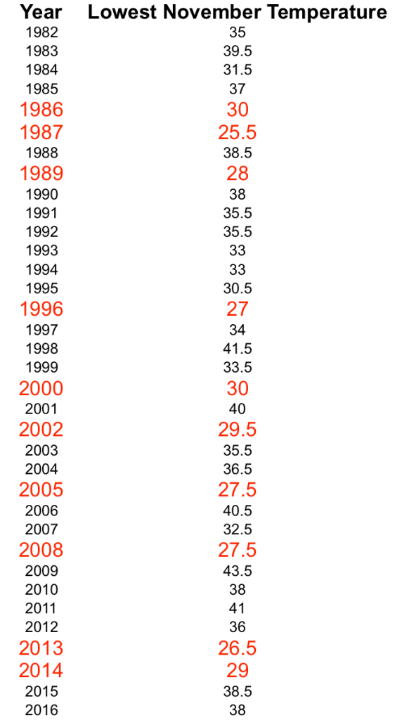
Success (Cold November) can happen in the first year, in which case X will be 1. We can see the success in the second year, in which case the sequence will be 01, and X will be 2 and so on.

In R, we can compute the probability P(X=1), P(X=2), etc., using the command dgeom. The Inputs are X and p. Try the following lines to create a visual of the distribution.

######################### GEOMETRIC DISTRIBUTION #########################

# The real data case # 
n = length(november_recent_coldtemp)

cold_years = which(november_recent_coldtemp <= 30)

ncold = length(cold_years)

p = ncold/n

x = 0:n
px = dgeom(x,p)
plot((x+1),px,type="h",xlab="Random Variable X (Cold on kth year)",ylab="Probability P(X=k)",font=2,font.lab=2)
abline(v = (1/p),col="red",lwd=2)
txt1 = paste("probability of cold year (p) = ",round(p,2),sep="")
txt2 = paste("Return period of cold years = E[X] = 1/p ~ 3.5 years",sep="")
text(20,0.2,txt1,col="red",cex=1)
text(20,0.1,txt2,col="red",cex=1)

Notice the geometric decay in the distribution. It can take X years to see the first success (or the next success from the current success). You must have seen that I have a thick red line at 3.5 years. This is the expected value of the geometric distribution. In lesson 34, we learned that the expected value of the geometric distribution is the return period of the event. On average, how many years does it take before we see the cold year again?

Did we answer the first two questions?

  1. Do you want to know what the probability of a cold November day is?
  2. Do you want to know what the return period of such an event is?

Suppose we want to compute the probability that the first success will occur within the next five years, we can use the command pgeom for this purpose.

pgeom computes P(X < 5) as P(X = 1) + P(X = 2) + P(X=3) + P(X = 4). Try it for yourself and verify that they both match.

Suppose the probability is higher or lower, how do you think the distribution will change?

For this, I created an animation of the geometric distribution with changing values of p. See how the distribution is wider for smaller values of p and steeper for larger values of p. A high value of p (probability of the cold November year) indicates that the event will occur more often; hence the trials to success are less in number. On the other hand, a smaller value for p suggests that the event will occur less frequently. The number of trials it takes to see the first/next success is more; creating a wider distribution.

Here is the code for creating the animation. We used similar code last week for animating the binomial distribution.

######## Animation (varying p) #########
# Create png files for Geometric distribution #

png(file="geometric%02d.png", width=600, height=300)

n = 35 # to mimic the sample size for november cold 
x = 0:n

p = 0.1
for (i in 1:5)
{
 px = dgeom(x,p)
 
 plot(x,px,type="h",xlab="Random Variable X (First Success on kth trial)",ylab="Probability P(X=k)",font=2,font.lab=2)
 txt = paste("p=",p,sep="")
 text(20,0.04,txt,col="red",cex=2)
 p = p+0.2
}
dev.off()

# Combine the png files saved in the folder into a GIF #

library(magick)

geometric_png1 <- image_read("geometric01.png","x150")
geometric_png2 <- image_read("geometric02.png","x150")
geometric_png3 <- image_read("geometric03.png","x150")
geometric_png4 <- image_read("geometric04.png","x150")
geometric_png5 <- image_read("geometric05.png","x150")

frames <- image_morph(c(geometric_png1, geometric_png2, geometric_png3, geometric_png4, geometric_png5), frames = 15)
animation <- image_animate(frames)

image_write(animation, "geometric.gif")

Negative Binomial Distribution

In lesson 35, we learned that the number of trials it takes to see the second success is Negative Binomial distribution. The number of trials it takes to see the third success is Negative Binomial distribution. More generally, the number of trials it takes to see the ‘r’th success is Negative Binomial distribution.

We can think of a similar situation where we ask the question, how many years does it take to see the third cold year from the current cold year. It can happen in year3, year 4, year 5, and so on, following a probability distribution.

You can set this up in R using the following lines of code.

################ Negative Binomial DISTRIBUTION #########################
require(combinat)

comb = function(n, x) {
 return(factorial(n) / (factorial(x) * factorial(n-x)))
}

# The real data case # 
n = length(november_recent_coldtemp)

cold_years = which(november_recent_coldtemp <= 30)

ncold = length(cold_years)

p = ncold/n

r = 3 # third cold year

x = r:n

px = NA

for (i in r:n)
{
 dum = comb((i-1),(r-1))*p^r*(1-p)^(i-r)
 px = c(px,dum)
}

px = px[2:length(px)]

plot(x,px,type="h",xlab="Random Variable X (Third Cold year on kth trial)",ylab="Probability P(X=k)",font=2,font.lab=2)

There is an inbuilt command in R for Negative Binomial distribution (dnbinom). I chose to write the function myself using the logic of the negative binomial distribution for a change.

The distribution has a mean of 10.5 years. The third cold year can occur approximately on the 10th year on average.

If you are comfortable so far, think about the following questions:

What happens to the distribution if you change r.

What is the probability that the third cold year will occur within seven years?

Poisson Distribution

Now let’s address the question: how many such events happened in the last five years?”

In lesson 36, Able and Mumble taught us about the Poisson distribution. We now know that counts, i.e., the number of times an event occurs in an interval follows a Poisson distribution. In our example, we are counting events that occur in time, and the interval is five years. Observe the data table and start counting how many events (red color rows) are there in each five-year span starting from 1982.

From 1982 – 1986, there is one event; 1987 – 1991, there are two events; 1992 – 1996, there is one event; 1997 – 2001, there is one event; 2002 – 2006, there are two events; 2007 – 2011, there is one event; 2012 – 2016, there are two events.

These counts (1, 2, 1, 1, 2, 1, 2) follow a Poisson distribution with an average rate of occurrence of 1.43 per five-years.

The probability that X can take any particular value P(X = k) can be computed using the dpois command in R.

Before we create the probability distribution, here are a few tricks to prepare the data.

Data Rearrangement

We have the data in a single vector. If we want to rearrange the data into a matrix form with seven columns of five years each, we can use the array command.

# rearrange the data into columns of 5 years #
data_rearrange = array(november_recent_coldtemp,c(5,7))

This rearrangement will help in computing the number of events for each column.

Counting the number of events

We can write a for loop to count the number of years with a temperature less than 30F for each column. But, R has a convenient function called apply that will perform this same analysis faster.

The apply command can be used to perform any function on the data row-wise, column-wise or both. The user can define the function.

For example, we can count the number of years with November temperature less than 30F for each column using the following one line code.

# count the number of years in each column with temp < 30
counts = apply(data_rearrange,2,function(x) length(which(x <= 30)))

The first argument is the data matrix; the second argument “2” indicates that the function has to be applied for the columns (1 for rows); the third argument is the definition of the function. In this case, we are counting the number of values with a temperature less than 30F. This one line code will count the number of events.

The rate of occurrence is the average of these numbers = 1.43 per five-year period.

We are now ready to plot the distribution for counts assuming they follow a Poisson distribution. Use the following line:

plot(0:5,dpois(0:5,mean(counts)),type="h",xlab="Random Variable X (Cold events in 5 years)",ylab="Probability P(X=k)",font=2,font.lab=2)

You can now tune the knobs and see what happens to the distribution. Remember that the tuning parameter for Poisson distribution is

I will leave you this week with these thoughts.

If we know the function f(x), we can find out the probability of any possible event from it. If the outcomes are discrete (as we see so far), the function is also discrete for every outcome.

What if the outcomes are continuous?

How does the probability distribution function look if the random variable is continuous where the possibilities are infinite?

Like the various types of discrete distributions, are there different types of continuous distributions?

I reminded you at the beginning that the autumn is ending. I am reminding you now that continuous distributions are coming.

If you find this useful, please like, share and subscribe.
You can also follow me on Twitter @realDevineni for updates on new lessons.

error

Enjoy this blog? Please spread the word :)